Figure 1: BPM system readout schematics (closed-orbit mode).
G. Garzoglio, K. E. Gollwitzer and G. Stancari
P-Bar Note #615
A new algorithm has been developed for the digital signal processor (DSP) in the digitizing card of the Accumulator beam position monitor (BPM) system. The main motivation is to make the measurement more accurate. The previous algorithm consisted of a fast Fourier transform (FFT) with a peak search; this was implemented only using 8192 samples. The algorithm presented here uses the ACNET value of the bunching RF frequency as an input parameter and so it only needs to perform a one-point Fourier transform. Moreover, a ping-pong mechanism for the management of the DSP memory has been implemented, which allows exploitation of a larger set of digitized data.

Figure 1: BPM system readout schematics (closed-orbit mode).
The signal from the BPM pick-up plates goes through a pre-amplifier mounted on the beam pipe at the location of the pick-ups. The pre-amplifiers also have a calibration input which can be used to determine a normalization between channels used by the DSP algorithm. After being brought up to the service building, the signal enters an analog down-converter (DC) card, which consists of an amplification stage and two low-pass filters (figure 1) for closed orbit measurements. Note that there is no down conversion done when the BPM system is in Closed Orbit Mode. The output of the DC card is fed to the digitizer card, which includes a sampling ADC and a DSP. A console application passes parameters to the DSP and reads the resulting position and amplitude measurements through the Slot 0 VXI Controller.
For every sector there is a VXI crate with four sets of analog and digitizing cards. Each set of cards consists of eight channels allowing for the determination of the position and amplitude for four BPMs. Each DSP is responsible for calculating the position for four BPMs. There are a total of 24 DSPs in the BPM system.
More information can be found
at http://
[3]www-rfi.fnal.gov/
[3]PBBPM/
[3]PBBPM.html.
In particular, information about ACNET control is documented.
The quantity of interest is the amplitude of the signal from each of
the pick-up plates of a BPM.
Let us first assume that, due to the RF bunching, the signal as a
function of time is described
by the function ![]() .
The first step of the algorithm (which we call ``heterodyne
method'' in analogy with the super-heterodyne radio receiver)
is to modulate the signal with a sine and a cosine of known
frequency
.
The first step of the algorithm (which we call ``heterodyne
method'' in analogy with the super-heterodyne radio receiver)
is to modulate the signal with a sine and a cosine of known
frequency ![]() (chosen to be as close as possible to
(chosen to be as close as possible to ![]() ):
):
![]()
![]()
The resulting functions ![]() and
and ![]() are the sum of a
low-frequency (
are the sum of a
low-frequency (![]() ) and a high-frequency
(
) and a high-frequency
(![]() ) component.
They are then integrated over a number n of periods of the
modulating frequency
) component.
They are then integrated over a number n of periods of the
modulating frequency ![]() :
:
![]()
![]()
The number n is chosen according to the following criteria:
![]()
in this way, the integration removes the high-frequency component
of ![]() and
and ![]() . The geometrical
average of the two integrals
. The geometrical
average of the two integrals ![]() and
and ![]() represents the
measurement of the signal amplitude A:
represents the
measurement of the signal amplitude A:
![]()
Multiplying the signal by both sine and cosine is done to get rid of
the initial phase ![]() . This procedure is equivalent to calculating
the modulus of the Fourier transform of the function
. This procedure is equivalent to calculating
the modulus of the Fourier transform of the function
![]()
at ![]() :
:

If the modulating frequency ![]() is not equal to
is not equal to ![]() ,
the measured amplitude
,
the measured amplitude ![]() is smaller than the
actual amplitude A.
Depending upon the desired precision on the measurement of the
amplitude, one can estimate a tolerable value for the frequency
difference
is smaller than the
actual amplitude A.
Depending upon the desired precision on the measurement of the
amplitude, one can estimate a tolerable value for the frequency
difference ![]() , what precision
, what precision ![]() must be known.
In the case of sinusoidal signal, the ratio
must be known.
In the case of sinusoidal signal, the ratio ![]() is given by the
following expression
(plotted in figure 4(a) as a function of
is given by the
following expression
(plotted in figure 4(a) as a function of ![]() for
for
![]() MHz, n = 3251 and
MHz, n = 3251 and ![]() rad):
rad):

Besides its obvious maximum at ![]() , this function has a
series of zeroes, the closest of which occur at
, this function has a
series of zeroes, the closest of which occur at ![]() . This is just a quantitative way of saying that
the wider the integration interval is, the more sensitive to a
frequency error the
amplitude measurement will be. Even when
. This is just a quantitative way of saying that
the wider the integration interval is, the more sensitive to a
frequency error the
amplitude measurement will be. Even when ![]() , there is an error if the integration extends over a
non-integer number of periods
, there is an error if the integration extends over a
non-integer number of periods ![]() (
(![]() ), but it is usually much smaller and decreases
rapidly as n increases. In the case of a sinusoidal signal, it can
be evaluated as follows:
), but it is usually much smaller and decreases
rapidly as n increases. In the case of a sinusoidal signal, it can
be evaluated as follows:
![]()

Figure 2: (a) The ratio B/A as a function of position x.
(b) Position error as a function of the ratio B/A for five
different values of the error ![]() on the ratio:
top curve
on the ratio:
top curve ![]() and bottom curve
and bottom curve ![]() .
.
To estimate how good the measurement of the amplitudes A and B on the two
pick-up plates has to be in order to get a reasonable position
accuracy, the relationship between the position x and the ratio r =
B/A has been analyzed![]() :
:
![]()
Figure 2(a)
emphasizes the dramatic change in amplitude ratio as the
position spans the available range.
An amplitude measurement error is parameterized by a factor ![]() (which will be, in general, a function of position) multiplying the
ratio r:
(which will be, in general, a function of position) multiplying the
ratio r: ![]() . Figure 2(b)
shows the position error
. Figure 2(b)
shows the position error ![]() as a function of r for different
values of
as a function of r for different
values of ![]() . As can be expected, the most stringent constraints
on accuracy come from positions near the center of the BPM. From the
same figure, one can deduce that if the ratio of the amplitudes is
measured with 5%
accuracy, the position error is always smaller than about 2%
of the full effective radius.
. As can be expected, the most stringent constraints
on accuracy come from positions near the center of the BPM. From the
same figure, one can deduce that if the ratio of the amplitudes is
measured with 5%
accuracy, the position error is always smaller than about 2%
of the full effective radius.
In reality, the BPM signal, instead of being a smooth function s(t),
consists of a string of ![]() integer numbers,
integer numbers, ![]() ,
in the range 0-4095, which come from the 12-bit sampling ADC
and are stored in the memory of the digitizer card.
The sampling frequency has been chosen to be
,
in the range 0-4095, which come from the 12-bit sampling ADC
and are stored in the memory of the digitizer card.
The sampling frequency has been chosen to be ![]() MHz,
so that each oscillation period of the signal contains
MHz,
so that each oscillation period of the signal contains ![]() sampling points (the RF is
sampling points (the RF is ![]() MHz, twice the
revolution frequency of the beam).
Therefore, each data set has information on approximately
MHz, twice the
revolution frequency of the beam).
Therefore, each data set has information on approximately ![]() oscillation periods.
In the DSP code, the measurement of the signal amplitude is achieved
through the following formula, in analogy with equation. 1:
oscillation periods.
In the DSP code, the measurement of the signal amplitude is achieved
through the following formula, in analogy with equation. 1:

The number NS is chosen in order to include the desired number of
complete oscillations; in our simulations and measurements it usually varies
between 8192
and 65536 (a memory hardware problem prevented us to use all of
the 131072 points). To save computing time, sines and cosines are
calculated only once and stored in a lookup table in the DSP memory. The
lookup table has 15000 entries, which are sufficient for representing
one period of a sinusoid with good numerical accuracy.

Figure 3: Diagram showing the averaging procedure.
An averaging feature has also been implemented (``video averaging'').
For a given total number NT of sampling points (which is usually
the maximum number of available data points 65536),
one can specify NS (![]() )
and the offset between samples NH (
)
and the offset between samples NH (![]() );
their meaning is explained in figure 3.
In this case, more than one amplitude measurement is performed,
one for each of the samples in figure 3; the
final result is the arithmetic mean of these measurements.
The purpose of the video averaging feature is to reduce the spread of
the position determination while keeping it independent from the
difference
);
their meaning is explained in figure 3.
In this case, more than one amplitude measurement is performed,
one for each of the samples in figure 3; the
final result is the arithmetic mean of these measurements.
The purpose of the video averaging feature is to reduce the spread of
the position determination while keeping it independent from the
difference ![]() (within a desired frequency range).
(within a desired frequency range).

Figure 4: Dependence of amplitude measurement on frequency,
for various values of the parameters.
The algorithm has been tested first by giving it a fake input data sample,
generated by a software signal simulator.
The simulator adds white noise![]() to a sinusoid of given amplitude, and
then discretizes the result, producing an ADC-like output (a set of
integer numbers).
Besides the signal and noise amplitudes, all the other parameters
(sampling and modulating frequency, number of data points, ...) can
be changed to see their effect.
to a sinusoid of given amplitude, and
then discretizes the result, producing an ADC-like output (a set of
integer numbers).
Besides the signal and noise amplitudes, all the other parameters
(sampling and modulating frequency, number of data points, ...) can
be changed to see their effect.
Figure 4 shows some of the results of the amplitude
measurements for the simulated signal.
The solid dots represent the output of the algorithm,
while the curves are the expected behavior as a function of ![]() (equation 2).
The signal amplitude A and the noise amplitude nA are in ADC
counts.
In the best case, when the amplitude is large compared to the LSB of
the ADC and there is no noise, the predicted amplitude is
identical to the measured amplitude, as shown in
figure 4(a).
Figure 4(b) confirms that integrating over a smaller number
of periods, the measured amplitude becomes less sensitive to the
frequency difference.
In figure 4(c) is shown the effect of discretization in
the ADC; the amplitude of the signal has been chosen to be only 5 ADC counts.
An amount of random noise comparable to the signal can compensate the
effects of discretization, as shown in figure 4(d).
Figure 4(e) illustrates that larger noise will
distort the results.
(equation 2).
The signal amplitude A and the noise amplitude nA are in ADC
counts.
In the best case, when the amplitude is large compared to the LSB of
the ADC and there is no noise, the predicted amplitude is
identical to the measured amplitude, as shown in
figure 4(a).
Figure 4(b) confirms that integrating over a smaller number
of periods, the measured amplitude becomes less sensitive to the
frequency difference.
In figure 4(c) is shown the effect of discretization in
the ADC; the amplitude of the signal has been chosen to be only 5 ADC counts.
An amount of random noise comparable to the signal can compensate the
effects of discretization, as shown in figure 4(d).
Figure 4(e) illustrates that larger noise will
distort the results.

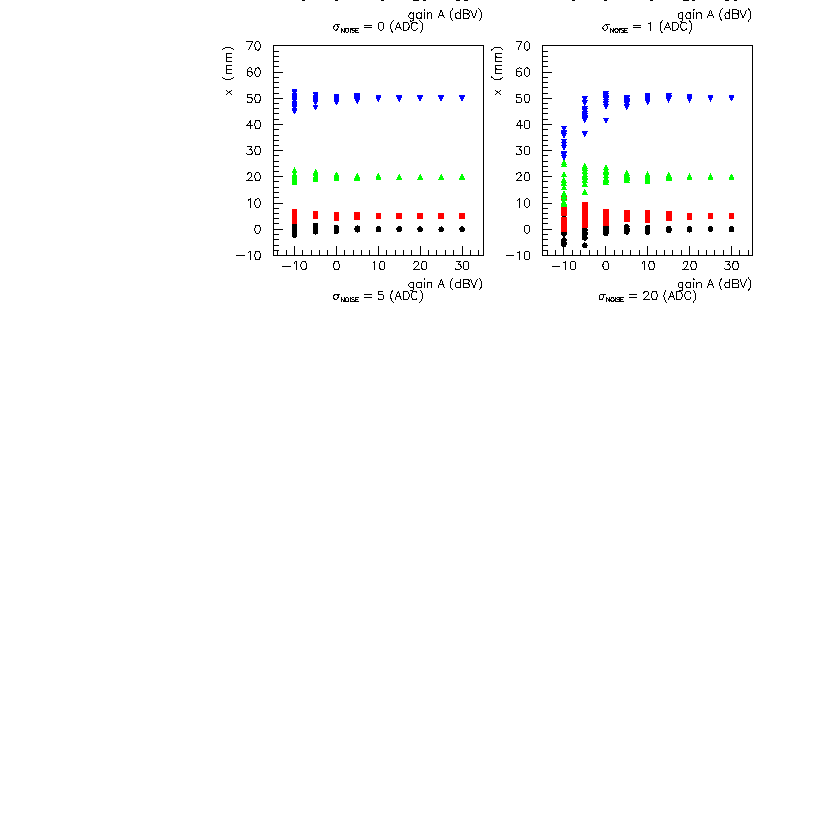
Figure 5: Results of the simulated position measurements.
The generated position was 0 mm (black dots), 5 mm (red squares), 20 mm
(green triangles pointing upwards) and 50 mm (blue triangles pointing
downwards).

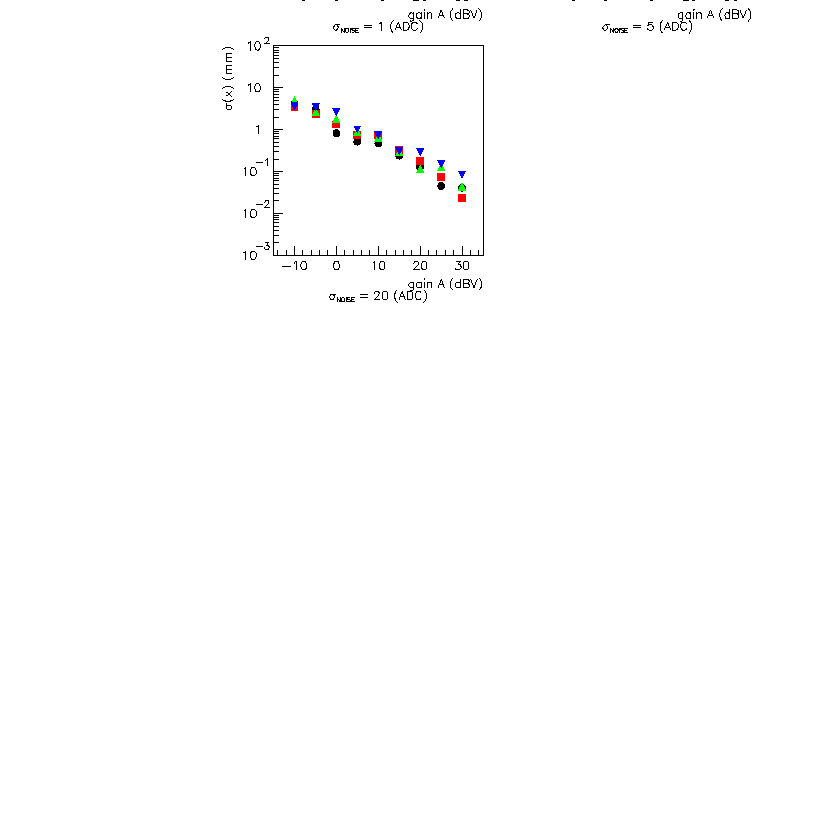
Figure 6: Standard deviation of the simulated position measurements.
The generated position was 0 mm (black dots), 5 mm (red squares), 20 mm
(green triangles pointing upwards) and 50 mm (blue triangles pointing
downwards).
The position measurement has also been simulated.
Four positions have been chosen (0 mm, 5 mm, 20 mm and 50 mm, with an
effective radius of 68 mm), and four noise amplitudes (0, 1, 5 and
20 ADC counts).
The software signal simulator generates a pair of signals
that would
give the desired position; this is done at nine different values of
the amplitude of the largest channel (channel A), from about 1 ADC count to
about 100 ADC counts (represented by the simulated gain of channel A going
from ![]() dBV to
dBV to ![]() dBV).
The pair of signals is the input of the heterodyne algorithm, which
outputs a measured position. The measured position is then compared
with the position generated by the simulator.
For each value of the above-mentioned parameters, twelve different pairs of
signals are generated, so that the spread of the results can be
evaluated.
Figure 5 shows the measured position as a function of
amplitude for the four different values of the noise amplitude;
for these plots,
dBV).
The pair of signals is the input of the heterodyne algorithm, which
outputs a measured position. The measured position is then compared
with the position generated by the simulator.
For each value of the above-mentioned parameters, twelve different pairs of
signals are generated, so that the spread of the results can be
evaluated.
Figure 5 shows the measured position as a function of
amplitude for the four different values of the noise amplitude;
for these plots, ![]() and
and ![]() .
The spread in the measurements is quantitatively
represented by the standard deviations in figure 6.
This simulation predicts that, if the white noise is small (say, 1 ADC
count) and the only other source of non-linearity is the ADC
digitization, the position can be determined to less than 0.3 mm
(using all the available data points
.
The spread in the measurements is quantitatively
represented by the standard deviations in figure 6.
This simulation predicts that, if the white noise is small (say, 1 ADC
count) and the only other source of non-linearity is the ADC
digitization, the position can be determined to less than 0.3 mm
(using all the available data points ![]() ).
).
Note that none of the simulations have any coherent noise. The actual environment has many sources of electronic noise.
The amount of DSP memory used for the algorithm memory
is limited to 192 KB.
The FFT algorithm only use the first 8192 samples.
This led to statistically poor measurements, with relatively large
fluctuations.
We decided to allocate memory for the sinusoid lookup table of
60 KB and for two ping-pong buffers with each having 60 KB.
While one buffer is being analyzed, the next subset of data is
transfered from the ADC's memory to the other ping-pong buffer in
the DSP algorithm memory area. The memory management is done so that it is
transparent to the amplitude measurement algorithm; in this way, a data sample
of any length can be analyzed in its entirety.
By going from 8192 to 65536 data points, for instance,
the fluctuations are
expected to be
reduced by a factor of ![]() .
.

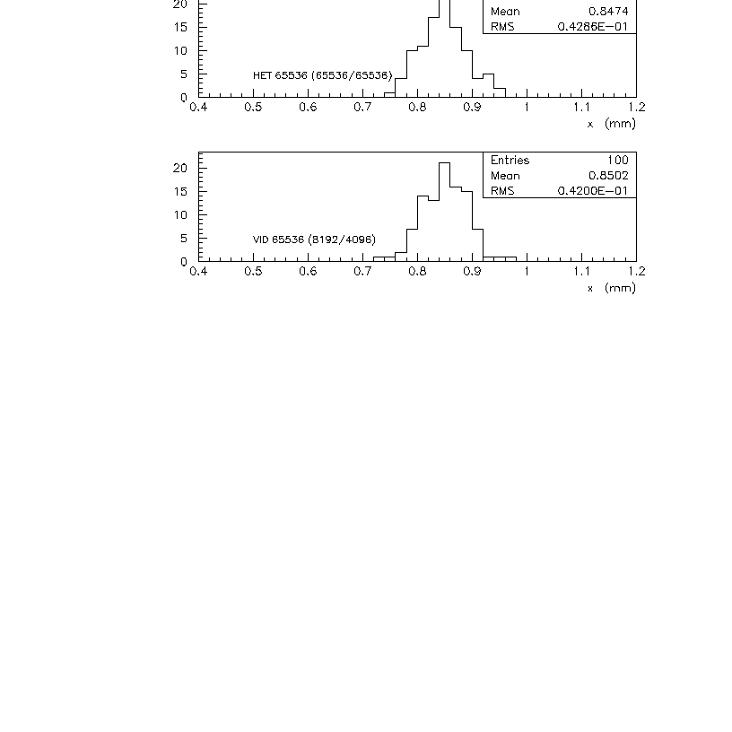
Figure 7: Calibration setup.
Comparison of position measurements from three algorithms.
Calibration signal of 50 mV and DC card gain set at -10 dBV.

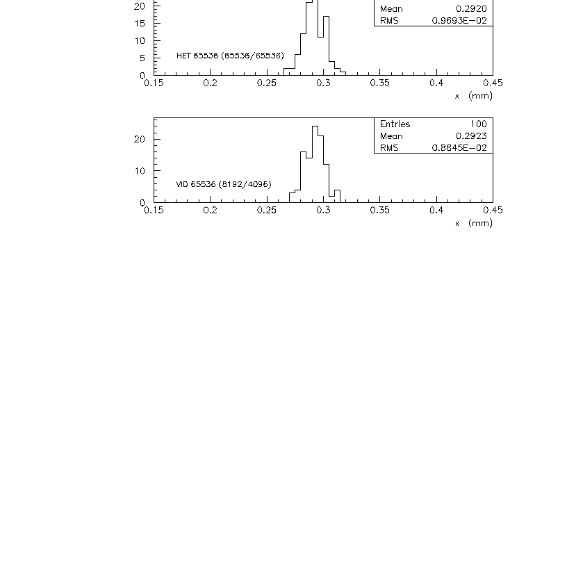
Figure 8: Calibration setup.
Comparison of position measurements from three algorithms.
Calibration signal of 250 mV and DC card gain set at -10 dBV.
The algorithm has been tested with the real readout hardware using the calibration system. It has also been compared with the FFT algorithm.
Figures 7
and 8 show the distribution of 100
position measurements from one BPM for different
intensities into the ADC,
respectively. The three histograms in each figure correspond to
the FFT algorithm, the heterodyne algorithm with ![]() ,
,
![]() and
and ![]() , and the heterodyne
algorithm with
, and the heterodyne
algorithm with ![]() ,
, ![]() and
and ![]() (VID is just the name of the heterodyne algorithm after the
addition of the video-averaging feature).
(VID is just the name of the heterodyne algorithm after the
addition of the video-averaging feature).
The algorithms' mean positions agree at each intensity. The rms spread decreases by better than a factor of 3.75 which is more than the expected decrease due to 8 times the statistics. For the new algorithm, the rms spread decreased from 0.04 mm to 0.01 mm when the signal intensity increased by a factor of 5.
Table 1 shows the length of time for the BPM system
to complete ten consecutive measurements.
The ARM and TRG clock events were set to 0F which means that the DSP
was in the IDLE or ARM state for ![]() second for the ten measurements.
It takes the same amount of time for
second for the ten measurements.
It takes the same amount of time for ![]() using the FFT and
HET algorithms.
The time is nearly linear with
using the FFT and
HET algorithms.
The time is nearly linear with ![]() when the HET algorithm is used.
The VID algorithm with no overlap (
when the HET algorithm is used.
The VID algorithm with no overlap (![]() ) is a little slower than
the HET algorithm for
) is a little slower than
the HET algorithm for ![]() .
The ratio of
.
The ratio of ![]() is the factor for the increase of time to
do the calculations from the no overlap case
(
is the factor for the increase of time to
do the calculations from the no overlap case
(![]() ) due to the increased number of
times that each point is used (simply more calculations are done).
) due to the increased number of
times that each point is used (simply more calculations are done).
A new algorithm has been successfully implemented with the DSPs of the
BPM system.
A FFT method has been replaced by a one-point Fourier transform.
The new algorithm uses a ping-pong method to access the ADC data.
Since the new algorithm uses more of the available ADC data, the new method
is more accurate.
The speed of the new and old algorithms are equivalent for the small data set
that had been used.
To have expanded the FFT data sample, the processing time should have
increased as ![]() ;
whereas the new algorithm processing time has been shown to go as
;
whereas the new algorithm processing time has been shown to go as ![]() .
The RF is needed by the new algorithm; the more accurate the better.
There is the option to
analyze the data in segments smaller than the total data set in order to
perform a video average.
This will be helpful if the RF is not known accurately.
Further tests will be performed when beam becomes available.
.
The RF is needed by the new algorithm; the more accurate the better.
There is the option to
analyze the data in segments smaller than the total data set in order to
perform a video average.
This will be helpful if the RF is not known accurately.
Further tests will be performed when beam becomes available.
DSP Algorithm for the Closed Orbit Analysis of the Signal from the Accumulator BPMs
This document was generated using the LaTeX2HTML translator Version 96.1-h (September 30, 1996) Copyright © 1993, 1994, 1995, 1996, Nikos Drakos, Computer Based Learning Unit, University of Leeds.
The command line arguments were:
latex2html -dir /wwwsrv/servers/e835/people/stancari/WWW/pbar/bpm/ -address stancari@fnal.gov note.tex.
The translation was initiated by Giulio Stancari on Thu Aug 19 11:31:59 CDT 1999